Overview
3DSNP is an integrated database for annotating the regulatory function of human noncoding SNPs by exploring their 3D interactions with genes and other SNPs mediated by chromatin loops. The models of cis-acting DNA elements regulating gene expression through three dimensional interactions mediated by chromatin loops have been established recently, and SNPs were reported frequently located in these elements. 3DSNP collects currently available Hi-C datasets from different studies. Two types of linkages were defined according to the spectrums of the loops: “Within Loop” or “Anchor-to-Anchor”. Allele frequencies were obtained for the SNPs in 1000 Genomes Phase 3 data, and pairwise LD was calculated for all pairs of SNPs in each continental population (EAS, AFR, AMR, ASN, EUR) within 200 kb. 3DSNP also integrated chromatin state segments, transcription factor binding sites and DNA accessibility from the Roadmap Epigenomics and ENCODE projects, DNA-binding motifs from TRANSFAC and JASPAR databases, eQTLs from the GTEx project and sequence conservation from UCSC Genome Browser. Visualization tools were developed for 3DSNP to display interacting SNPs, genes and elements along with important epigenetic marks, and a comprehensive scoring system was developed to assess the functionality of SNPs in different aspects. 3DSNP provides an integrated database and visualization tools for discovering the regulatory roles of noncoding SNPs mediated by 3D genome topology.
Data source
Sequential and genotyping data
3DSNP contains all 149,254,102 SNPs and small indels from NCBI dbSNP build 146. Among them, 84,801,880 SNPs were phased using 1000 Genomes Project Phase 3 (final phase) genotype data, the allele frequencies were obtained and pairwise LD was calculated for all pairs of SNPs in each continental population (AFR, AMR, ASN, EUR and SAS) within 200 kb. In addition, minor allele frequency (MAF) and linear closest gene were also extracted from dbSNP. Gene annotations were obtained from GRCh37/hg19 version of RefSeq genes from the UCSC Genome Browser.
3D genome topology
Chromatin loops identified by Hi-C technology in multiple human cell types were collected from published Hi-C studies (Rao et al. 2015, Sanborn et al. 2015, Taberlay et al. 2016) to map the intrachromosomal interactions between distant genomic regions. In total, 3DSNP collected 75,362 intrachromosome chromatin loops in twelve human cell types. It has been reported that Chromatin interactions are classified into two types based on the spans of chromatin loops. For a chromatin loop shorter than 200 kb, the corresponding interaction type is ‘Within loop’, where genomic elements located within can interact each other. For a chromatin loop longer than 200 kb, the type is ‘Anchor-to-anchor’, where only elements located at the two anchors are supposed to interact with each other.
Chromatin signature
A variety of chromatin signatures were used to annotate the regulatory functions of SNPs, including chromatin state (ChromHMM Core 15-state model), histone modifications (NarrowPeak), DNase I hypersensitivity sites and transcription factor binding sites from Roadmap Epigenomics and ENCODE projects. To annotate SNPs that alters TF binding motifs, TFM-Scan software was used to locate the putative TFBS across the genome using a set of position weight matrices (PWMs) collected from TRANSFAC and JASPAR databases.
Conservation
The conservation of SNPs was measured by two PhyloP scores obtained from the UCSC Genome Browser. The two PhyloP scores were calculated from multiple alignments of 46 vertebrate genomes and 33 mammal genomes respectively. The absolute values of the PhyloP scores represent -log(P-values) under a null hypothesis of neutral evolution, and sites predicted to be conserved are assigned positive scores, while sites predicted to be fast-evolving are assigned negative scores.
eQTL
Correlations between genotype and tissue-specific gene expression levels will help annotate the effects of genetic variants on gene regulation. We collected a total of 19,582,729 significant SNP-gene pairs (FDR <= 0.05) in 44 human tissues from the GTEx project version 6. To measure the significance of the eQTLs, nominal eQTL p-values and the effect size were obtained for each SNP-gene pair. Nominal eQTL p-values were generated using a two-tailed t test, testing the alternative hypothesis that the beta deviates from the null hypothesis of beta=0. The effect size of the eQTLs is defined as the slope (‘beta’) of the linear regression, and is computed as the effect of the alternative allele (ALT) relative to the reference allele (REF) in the human genome.
Visualization
Regional LD plot
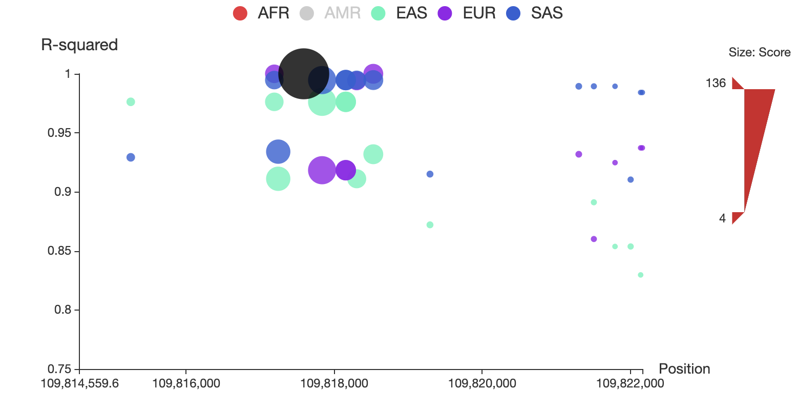
A regional plot is used to display a set of SNPs associated to the query in LD, as shown in Figure 1. In this plot, the x-axis shows chromosome coordinates, y-axis shows values for r2, the size of the node represents its total score, and associated SNPs in five populations are shown in different colors. Associated SNPs in each of the five populations can be removed from or added to the plot by clicking the corresponding circle in the legend. Users can also restrict the range of total score for displaying by adjusting the upper and lower bound of size bar at the right side of the plot. A detailed page will be opened by clicking the node of the corresponding SNP. The regional LD plots can be displayed in the browser and can also be downloaded as high quality, publication-ready PNG files.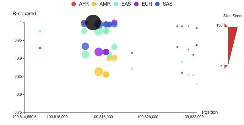
Figure 1. Regional LD plot of the associated SNPs of rs12740374. In the plot, x-axis shows chromosome coordinates, y-axis shows values for r2, the size of the node represents its total score, and associated SNPs in five populations (AFR: African, AMR: Ad Mixed American, ASN: East Asian, EUR: European and SAS: South Asian) are displayed in different colors, and rs12740374 is displayed in black.
CIRCOS plot
Circos is a software package for visualizing genomic data and information. A customizable Circos plotting system was developed to display the 3D chromatin topology and a set of important chromatin marks surrounding the query SNP. Circos tracks from outside to inside represent: Chromatin states, RefSeq genes, DHS and histone modifications, TFBS, associated SNPs and chromatin loops, as shown in Figure 2. The color scheme of 15 chromatin states in ChromHMM model is shown in Table 1, and the color scheme of chromatin loops in twelve cell types is shown in Table 2 below.
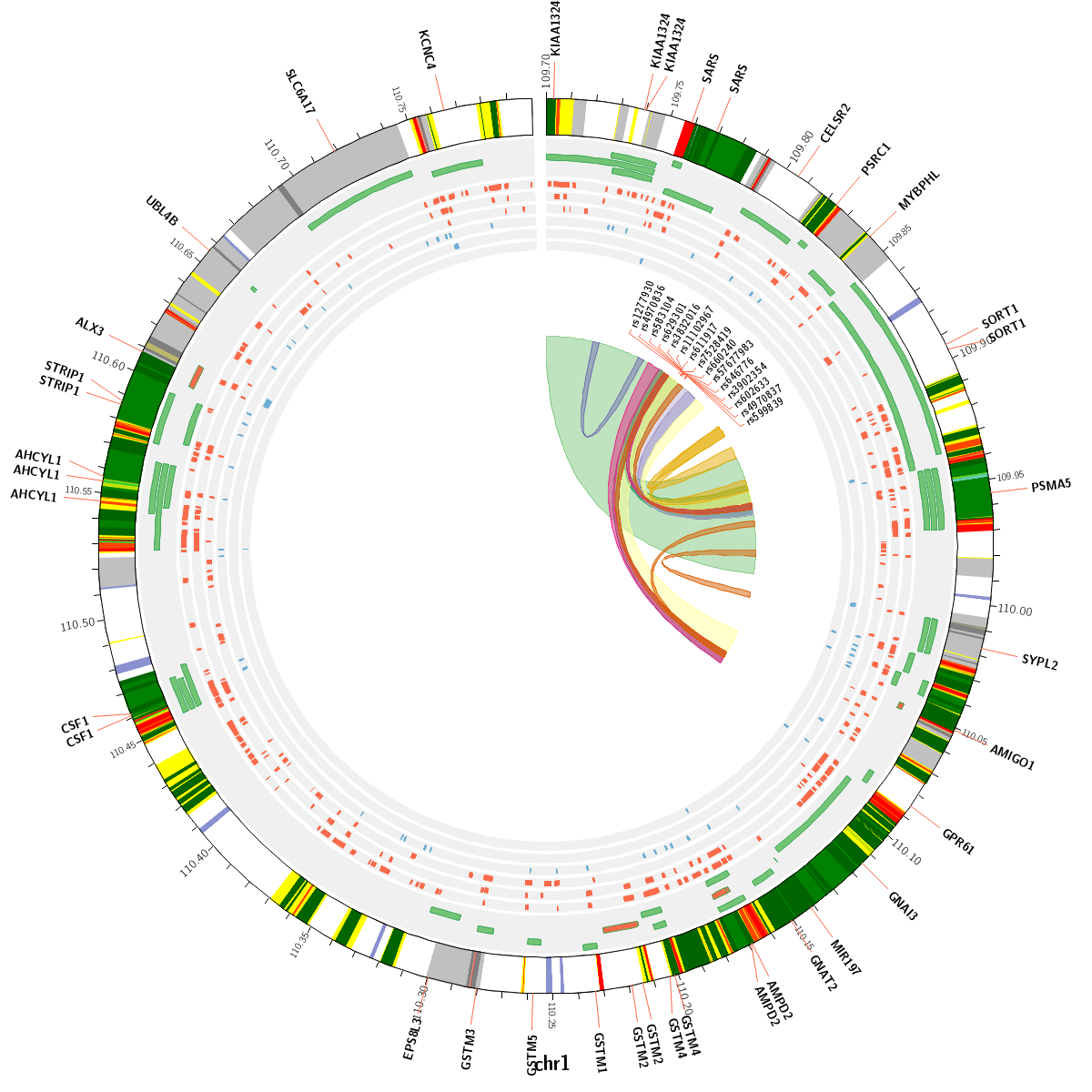
Figure 2. Track annotation for Circos plot. In the plot, from outer to inner, the circle represents chromatin states, annotated genes, histone modification set (red), transcription factor set (blue), current SNP and associated SNPs, and 3D chromatin interactions, respectively.
Table 1. Color scheme of 15 chromatin states in ChromHMM core model
| Color | State NO. | Mnemonic | Description |
|---|---|---|---|
| 1 | TssA | Active TSS | |
| 2 | TssAFlnk | Flanking Active TSS | |
| 3 | TxFlnk | Transcr. at gene 5′ and 3′ | |
| 4 | Tx | Strong transcription | |
| 5 | TxWk | Weak transcription | |
| 6 | EnhG | Genic enhancers | |
| 7 | Enh | Enhancers | |
| 8 | ZNF/Rpts | ZNF genes & repeats | |
| 9 | Het | Heterochromatin | |
| 10 | TssBiv | Bivalent/Poised TSS | |
| 11 | BivFlnk | Flanking Bivalent TSS/Enh | |
| 12 | EnhBiv | Bivalent Enhancer | |
| 13 | ReprPC | Repressed PolyComb | |
| 14 | ReprPCWk | Weak Repressed PolyComb | |
| 15 | Quies | Quiescent/Low |
Table 2. Color scheme of twelve cell types for the chromatin loop track in Circos plot
| Color | Cell type | Description | Tissue |
|---|---|---|---|
| GM12878 | Lymphoblastoid Cells | Blood | |
| K562 | K562 leukemia Cells | Blood | |
| H1-hESC | Embryonic stem cells | ESC | |
| IMR90 | Fetal lung fibroblasts | Lung | |
| HeLa-S3 | Cervical carcinoma cells | Cervix | |
| HUVEC | Umbilical vein endothelial cells | Blood vessel | |
| NHEK | Epidermal keratinocytes | Skin | |
| HMEC | Mammary epithelial cells | Breast | |
| KBM-7 | Chronic myelogenous leukemia (CML) cells | Blood | |
| LNCaP | Prostate adenocarcinoma | Prostate | |
| PC3 | Prostate cancer cells | Prostate | |
| PrEC | Prostate epithelial cell line | Prostate |
You can customize the Circos tracks in the ‘Options’ block to display DHS, histone modifications of 127 cell lines in Roadmap Epigenomics Project and the binding sites of CTCF and other 166 transcription factors of 91 cell lines in ENCODE Project. The DHS and histone modification track is represent by red tiles and TFBS is represent by blue tiles.
UCSC Genome Browser plot
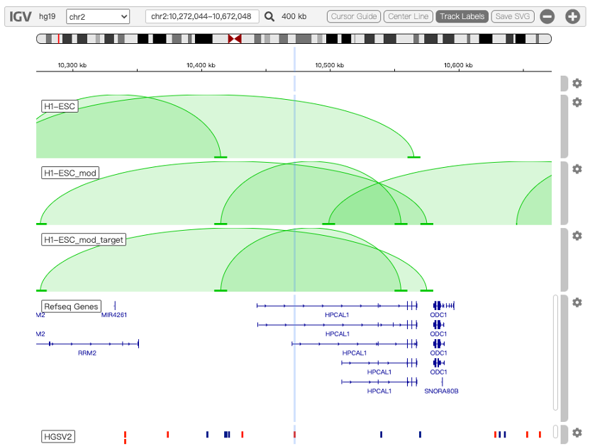
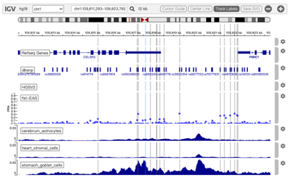
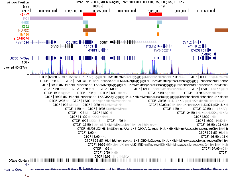
Chromatin loops and chromatin signatures surrounding the query SNP can be also displayed in a figure generated by the UCSC Genome Browser with custom tracks. The location of the query SNP is marked by red bar, and pairs of anchor sites of chromatin loops are displayed with colored bars for different cell types, as shown in Figure 3.
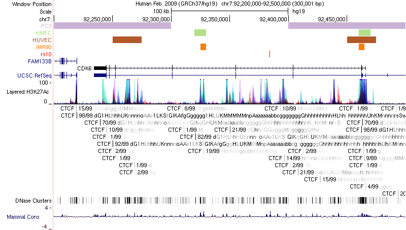
Figure 3. Track annotation for UCSC Genome Browser plot. In the plot, from top to bottom, the tracks are: genomic coordinates, chromatin interactions, current SNP, UCSC genes, RefSeq genes, histone modifications, CTCF binding sites, DNase Clusters and mammal conservation.
Scoring system
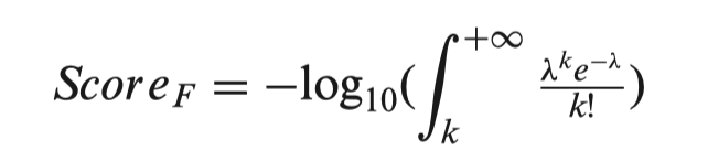
In 3DSNP, each SNP is scored based on its annotated records on six functional categories: 3D interacting genes, Enhancer state, Promoter state, Transcription factor binding sites, sequence motifs altered and conservation score. Different from the scoring scheme of RegulomeBD, which classifies SNPs into classes based on the combinatorial presence/absence status of functional categories, 3DSNP adopts a quantitative scoring system to evaluate the functional significance of a SNP in different categories. For the first five categories, we used the number of annotated records (hits) to assign score to a SNP in the corresponding category. Specifically, we fitted the numbers of hits of all SNPs in each chromosome to a Poisson distribution model. Considering a SNP has k hits in one functional category F, λ is the fitted parameter of the corresponding Poisson model, then the score of the SNP in this category is defined as follows:
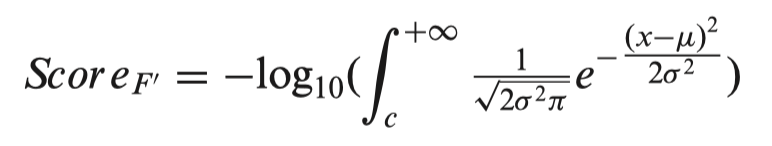
For the conservation category (F’), we found the PhyloP scores of all SNPs in a chromosome follow a Gaussian distribution. Considering a SNP has a conservation score of c, μ and σ are the fitted parameters of the corresponding Gaussian model, then the score of the SNP in the conservation category is defined as follows:
The total score of a SNP is the sum of scores of the six functional categories.
Data format
Query format
SNP ID(s), a single genomic region or an official gene symbol can be used as query to search the database by the search bar on the main page. Multiple SNP ids should be delimited by commas or spaces, a genomic region should be written as chrN:start-end, and a gene should be written as gene:SYMBOL. Only one query type is allowed for each searching and mixed query format is not supported. The maximum size of the query in the search bar is 100 SNP IDs.
Upload file format
A text file containing a list of SNP IDs or genomic regions can be uploaded to the server for batch analysis by clicking the browser icon at the right side of the search bar. The maximum size of SNPs in the file for uploading is 2000 SNPs, the maximum number of regions in the file is 10 regions, and any data exceeding the limitations will be ignored.
Export format
All resulting forms can be exported in three formats: copy to clipboard, MS excel or PDF and figures can be exported in PNG format.
Usage example
Type the full id “rs12740374” in the search box then the SNP rs12740374 will appear automatically in the main table below. You can see the position and reference/alternative sequence in the genome. The total functionality score of rs12740374 is 135.06, and its 3D interacting genes are PSRC1 and other 7 genes. Click the “+” icon on the left side of the ID to see a table containing a set of associated SNPs in the same LD block with rs12740374. A regional LD plot on the right side of the table shows their associations as below:

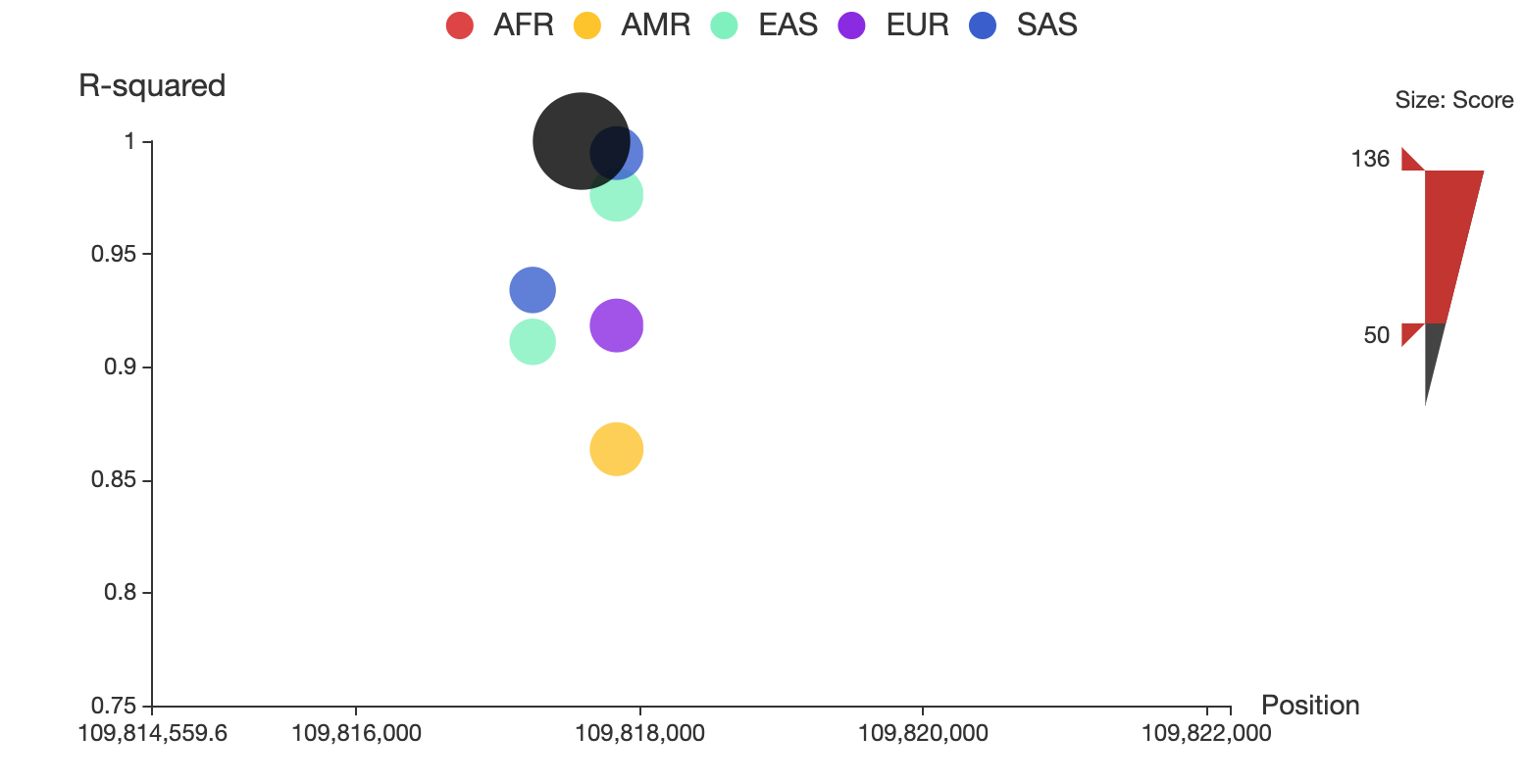
Click the “AMR” circle in the legend to remove the associated SNPs in AMR population, as shown below:
You can also restrict the range of total score for displaying by adjusting the upper and lower bound of size bar at the right side of the plot. For example, you can make it only show SNPs whose total score > 50 as below:
You can alway click on the node to see the details of the specific SNP in a new detailed page.
Then, click the SNP ID “rs12740374” will open a new page containing all detailed information about this SNP, which contains:
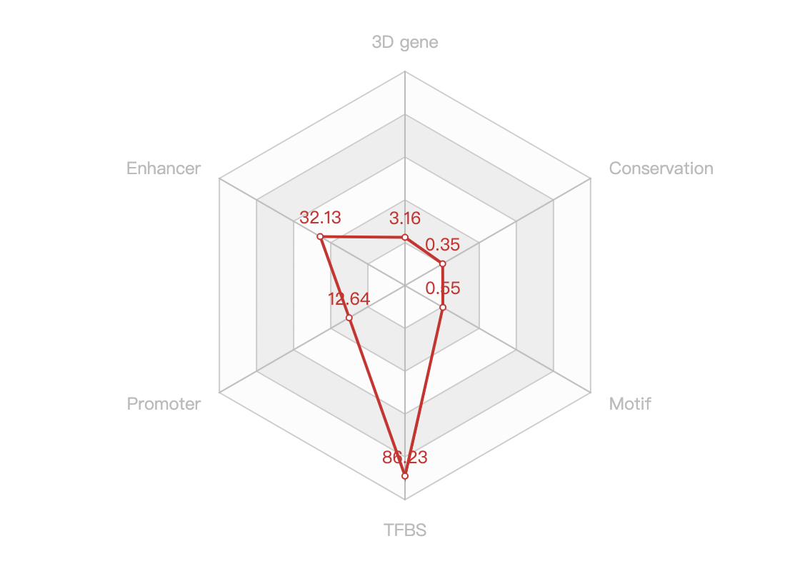
- A text paragraph summarizing it scores of the non-empty functional categories and a radar chart showing the distribution of the six scores, as below:
- A Circos plot showing the chromatin loops and other 2D signatures:
You can switch the cell type of the CIRCOS plot to another cell type in the ‘Options’ block. For example, you can change the cell type to HepG2 of the liver tissue, as shown below.

- A figure generated by UCSC Genome Browser with custom data:
- And a series of tables containing the details of 3D interacting genes, 3D interacting SNP, Chromatin state, TFBS and Conservation.