CommPath: inference and analysis of intercellular communications by pathway analysis
Overview
Here, we introduce CommPath, an open source R package and a webserver, to infer and visualize the LR associations and signaling pathway-driven cell-cell communications from scRNA-seq data.
Key Features
CommPath has two key features:
(i) it manually curates a comprehensive signaling molecule interaction database of LR interactions, as well as their currently accessible pathway annotations, including KEGG pathways, WikiPathways, reactome pathways, and GO terms;
(ii) it prioritizes both LR pairs among cell types and cell type specific signaling pathways mediating cell-cell communications.
Interface
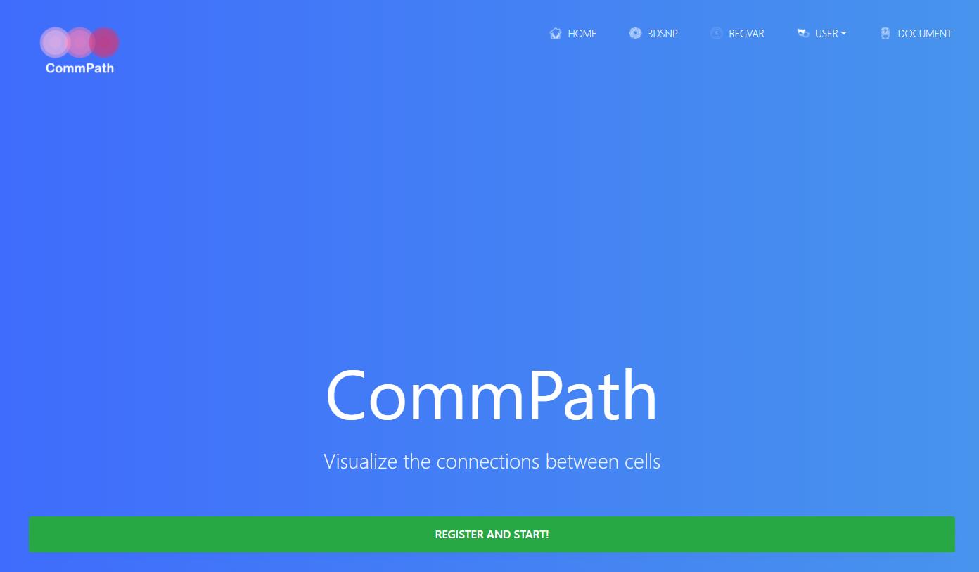
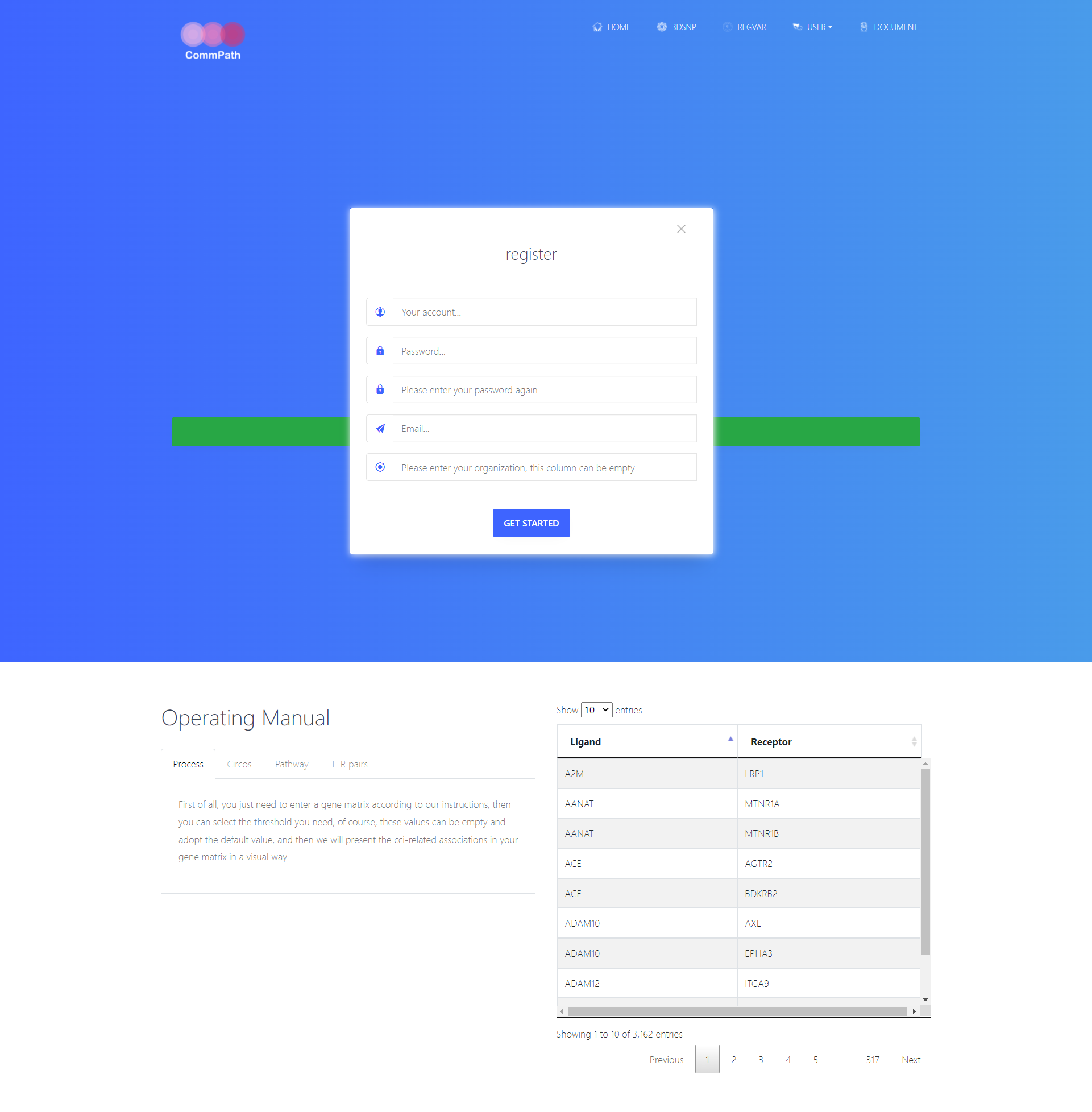
0.Register and login
CommPath needs to be registered. And through your CommPath account, you can easily get the analysis states and the results of your tasks.
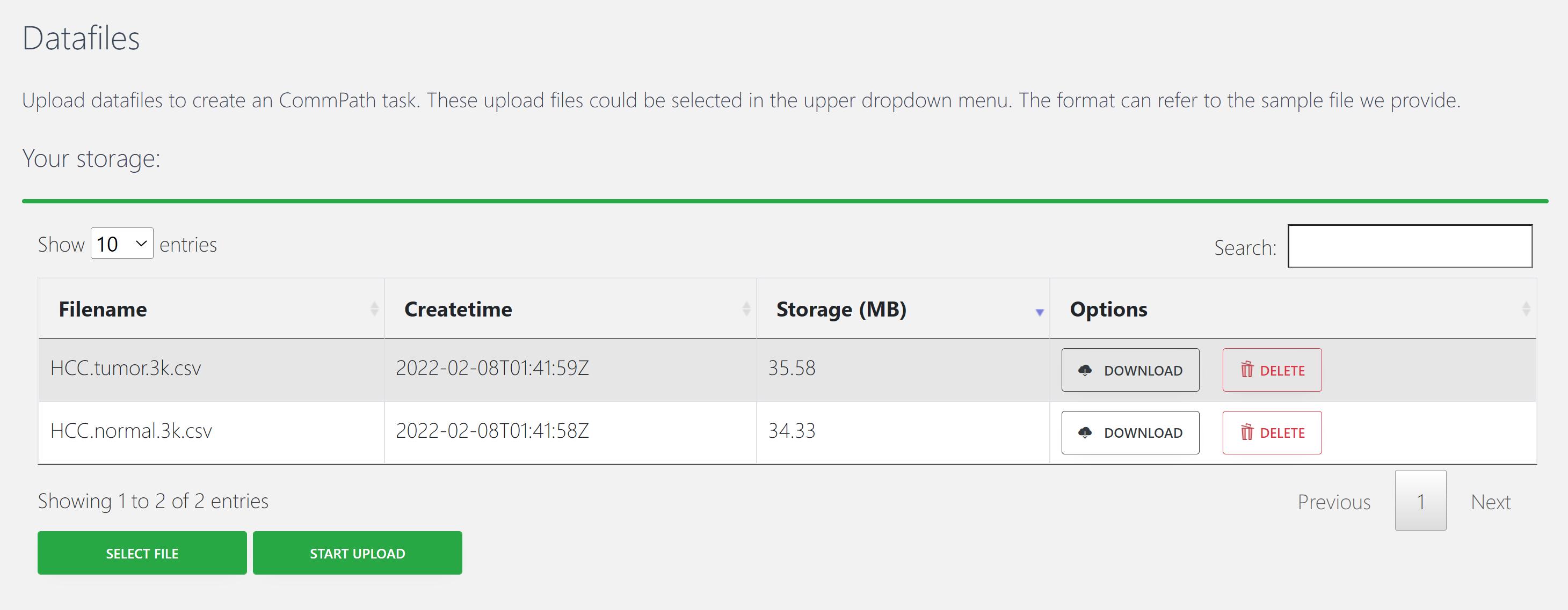
1. Upload input files
CommPath requires input of an expression matrix of gene × cell produced from scRNA-seq experiments and a label vector indicating cell clusters.
For example, here are N genes * M cells for P clusters (one row = one cell) with headers:
| Cells | Gene1 | Gene2 | …… | GeneN | Clusters |
|---|---|---|---|---|---|
| Cell1 | Cluster1 | ||||
| Cell2 | Cluster1 | ||||
| Cell3 | Cluster2 | ||||
| …… | …… | ||||
| CellM | ClusterP |
An example of input file is “HCC.tumor.3k.csv”.
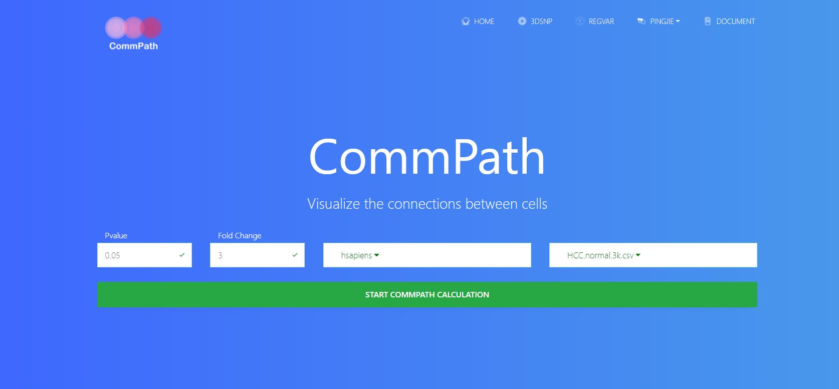
2. Run your task
To run a task, four parameters should be selected. These parameters are:
(1) Pvalue. Default = 0.05;
(2) Fold Change. Default = 3;
(3) Species. Now CommPath supports L-R pairs in 3 species, including human (hsapiens), mouse (mmusculus), and rat (rnorvegicus). More model organisms will be supported soon.
(4) Data files, which is your input file in “1. Upload input files” section.
And, click “START CommPath CALCULATION” to run a task.
Then, CommPath will automatically jump to “Task list” section, and the top row shows the task status in real time.
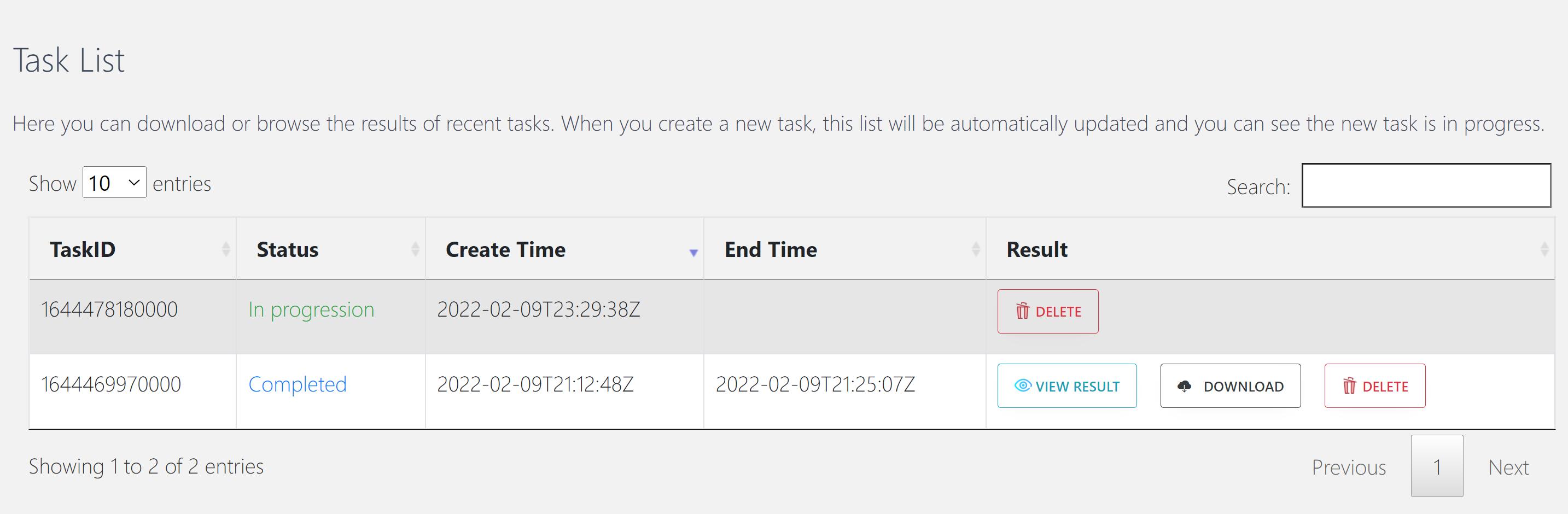
When the task status changed from “In progression” to “Completed”, you can click “VIEW RESULT” and browse the results.
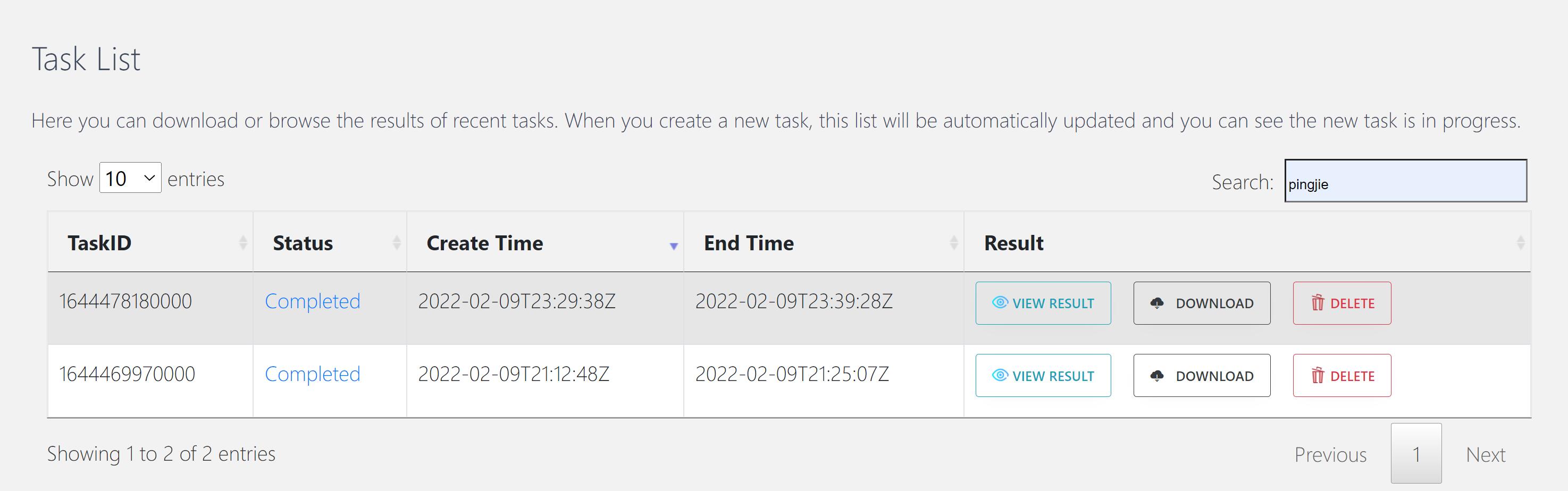
In the “Task list” section, you can also review the results of previously completed tasks.
3. Results
Results for all clusters
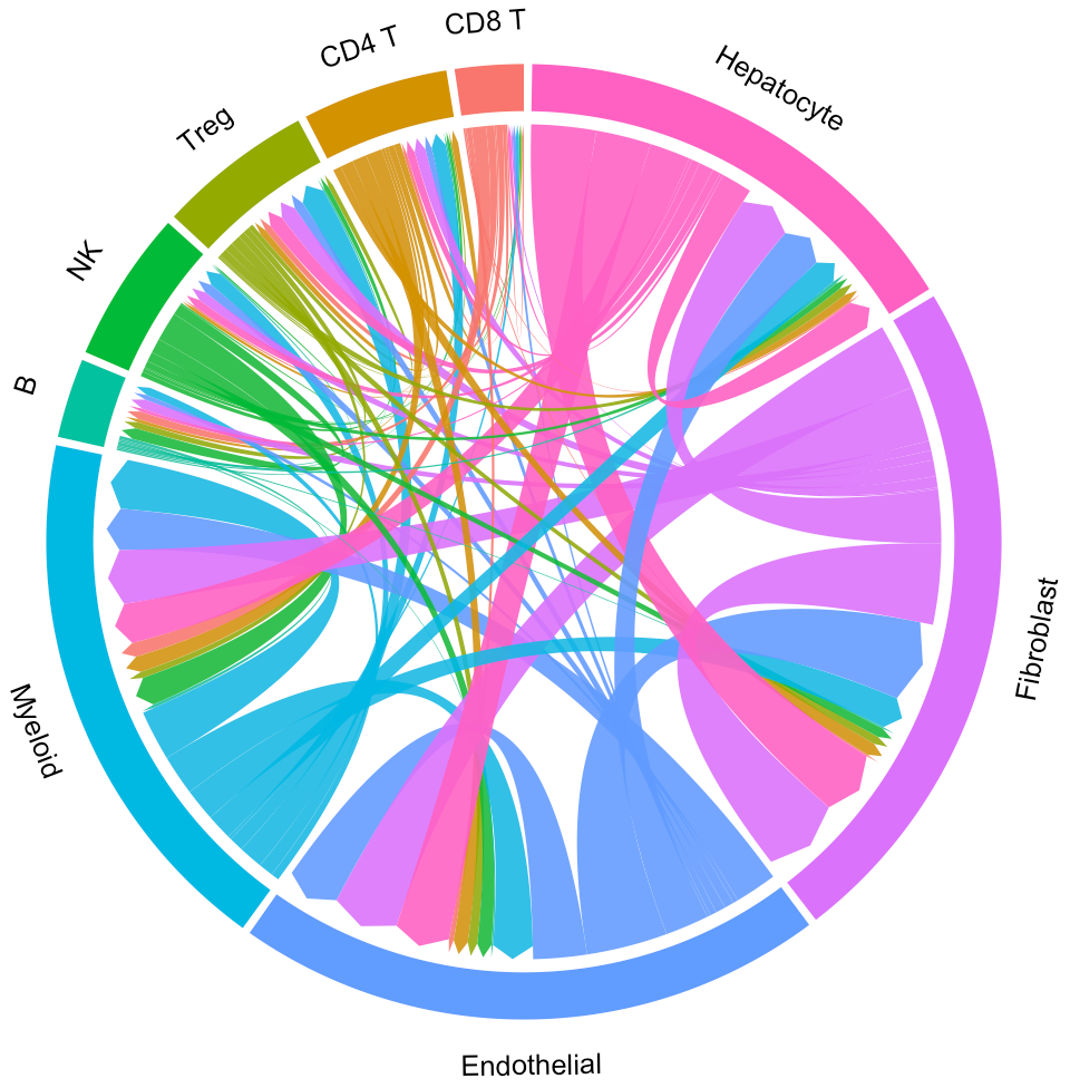
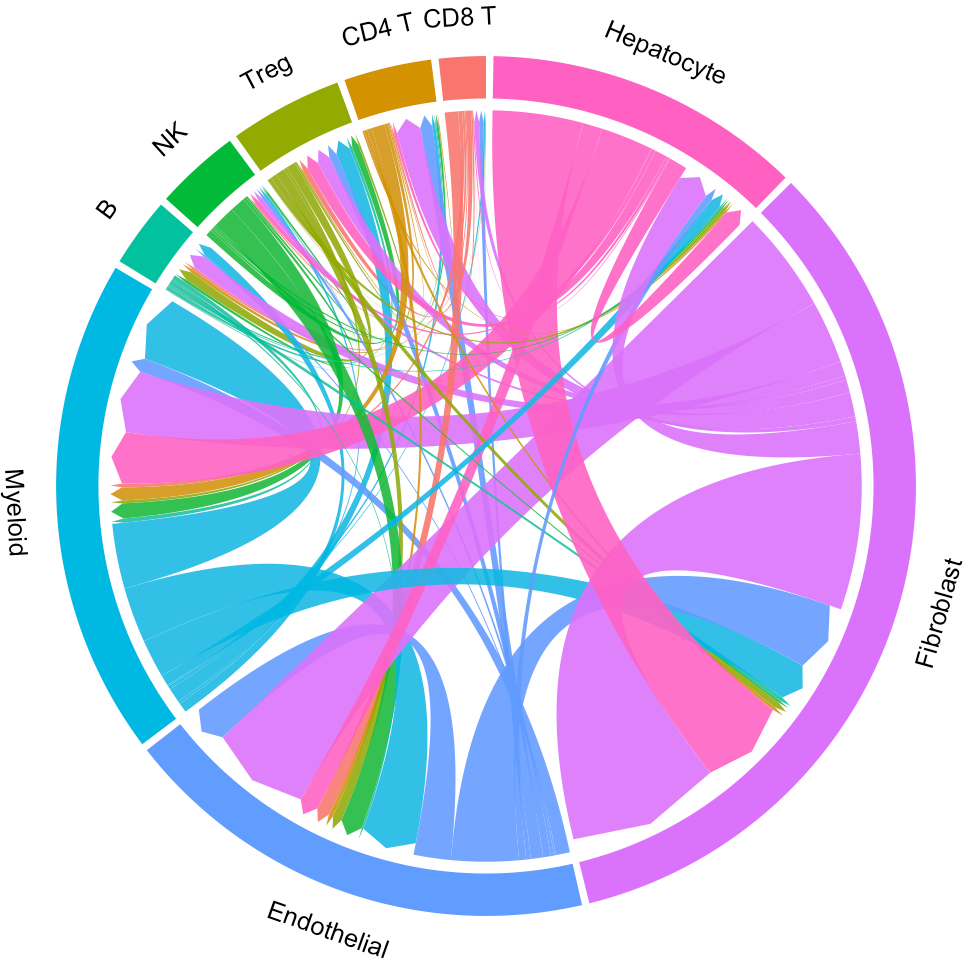
Default “Results” page (“Circos” tab page) shows circos of all clusters. The widths of lines indicate the counts (Left plot) or the overall interaction intensity (Right plot) of LR pairs among clusters.
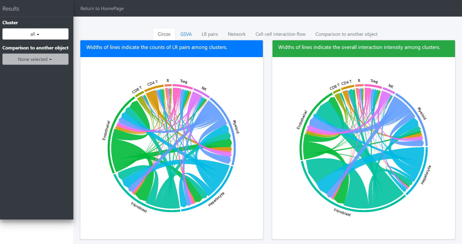
In the above circos plot, the directions of lines indicate the associations from ligands to receptors, and the widths of lines represent the counts of LR pairs among clusters.
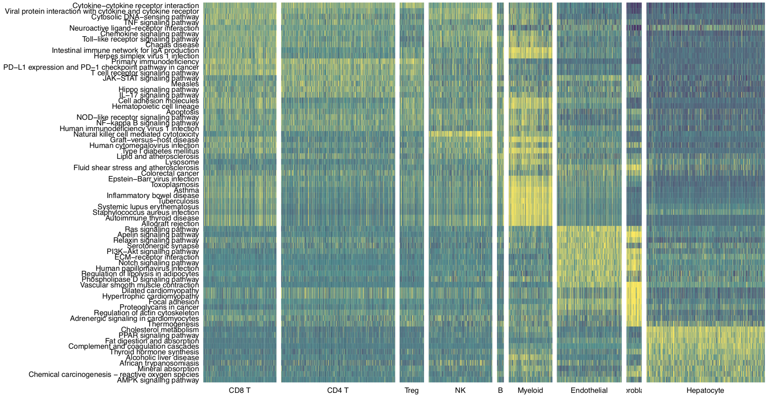
Pathway enrichment analysis
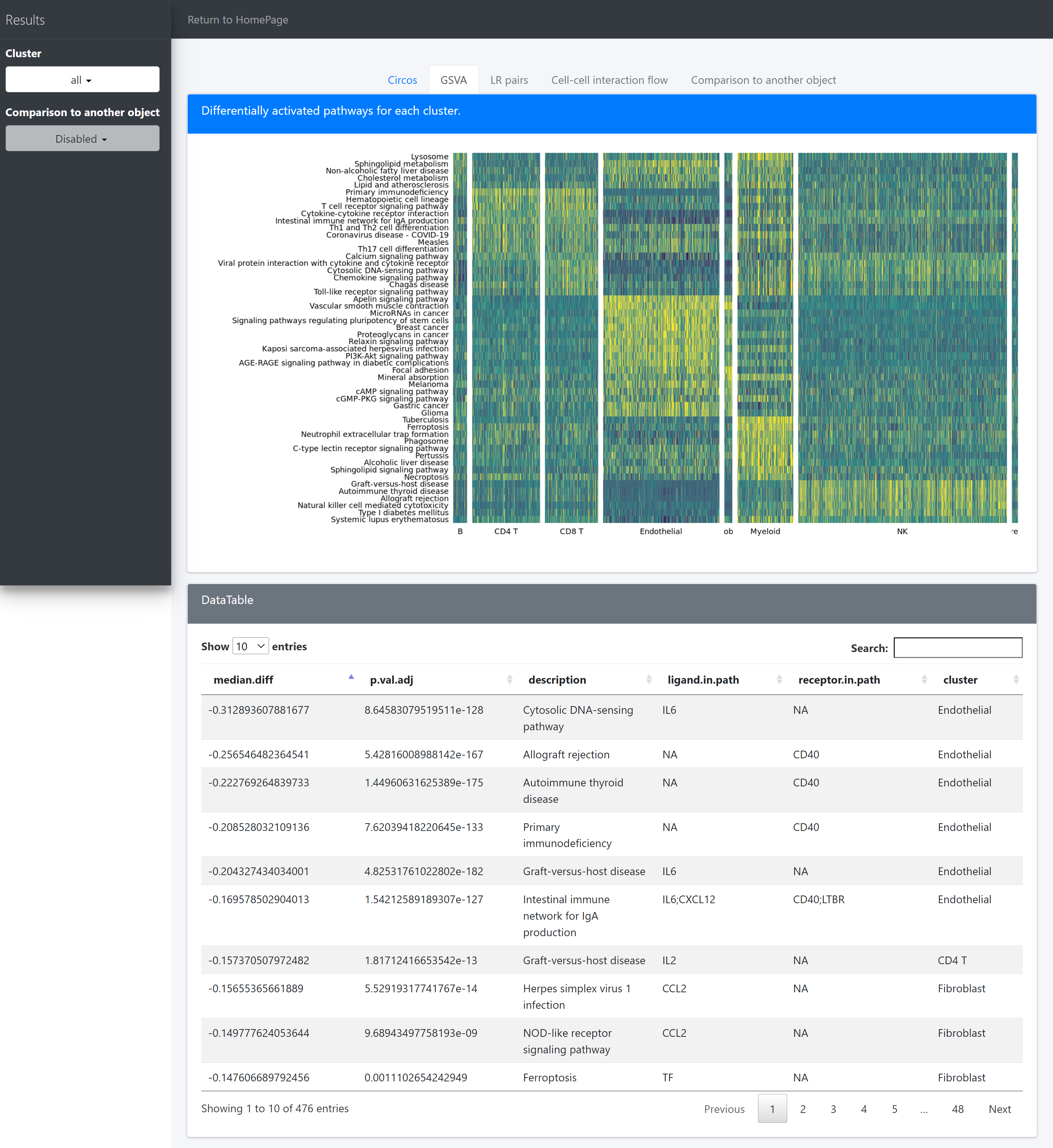
CommPath conducts pathway analysis to identify dysregulated signaling pathways containing the marker ligands and receptors for each cluster.
The “GSVA” tab page, shows differentially activated pathways for each cluster.
There are 7 columns stored in the variable ident.up.dat/ident.down.dat:
Columns cell.from, cell.to, ligand, receptor show the upstream and dowstream clusters and the specific ligands and receptors for the LR associations;
Columns log2FC.LR, P.val.LR, P.val.adj.LR show the interaction intensity (measured by the product of log2FCs of ligands and receptors) and the corresponding original and adjusted P values for hypothesis tests of the LR pairs or the overall interaction intensity among clusters.
Results for specific cluster
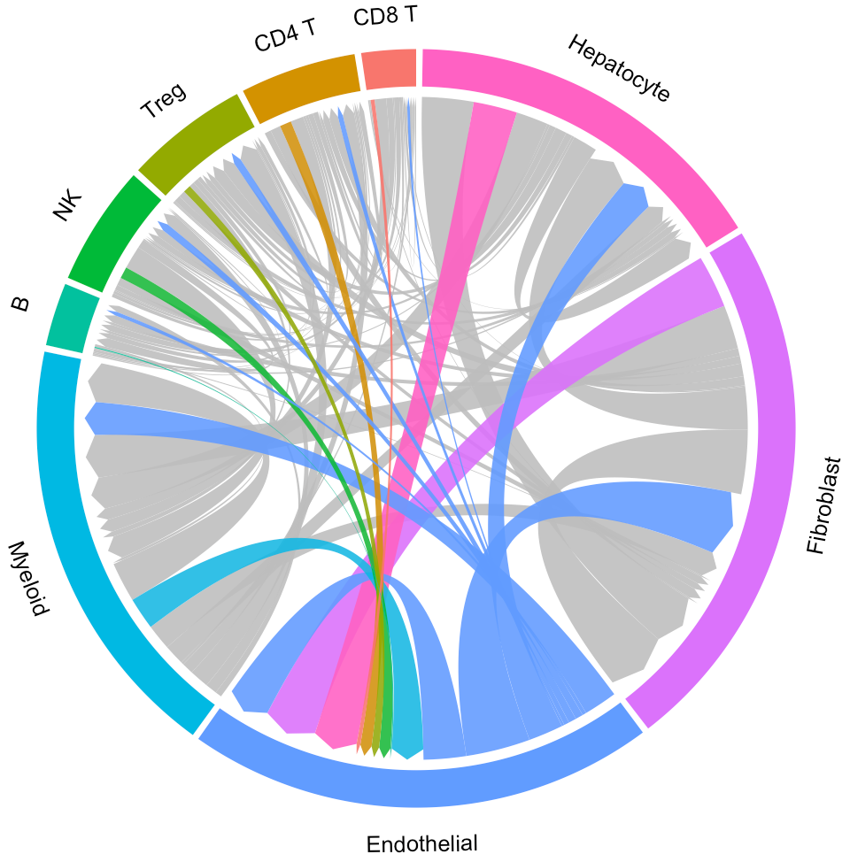
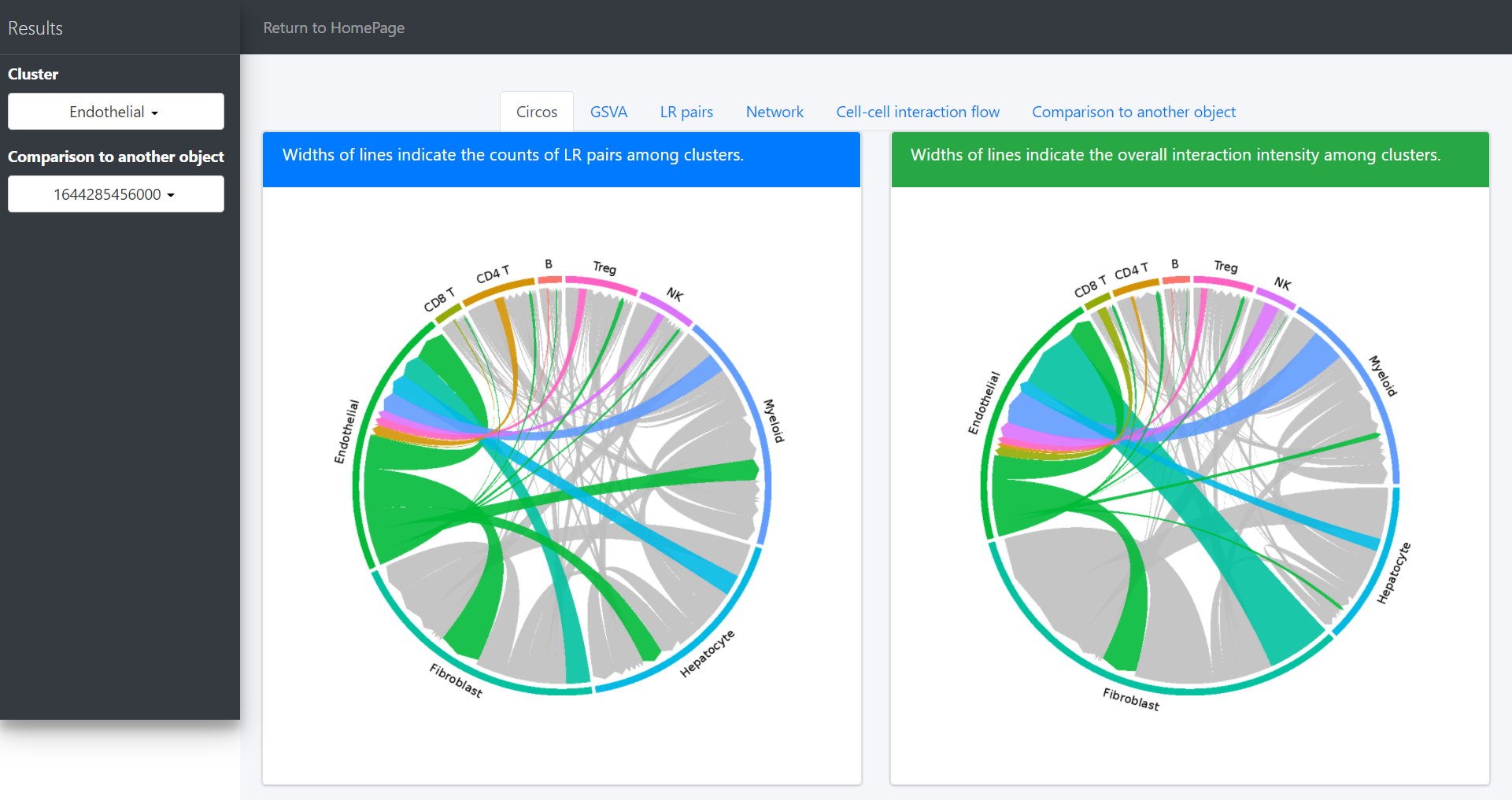
When you focus on some specific cluster (eg. Endothelial), you can select “Endothelial” on the “Cluster” drop-down menu. Then, the circos plot of “Endothelial” will update in “Circos” tab page, as well as L-R associations and signaling pathway-driven cell-cell communications (“LR pairs” tab page).
In the “Circos” tab page, users would highlight the interaction of specific clusters. Here we take the Endothelial cells as an example:
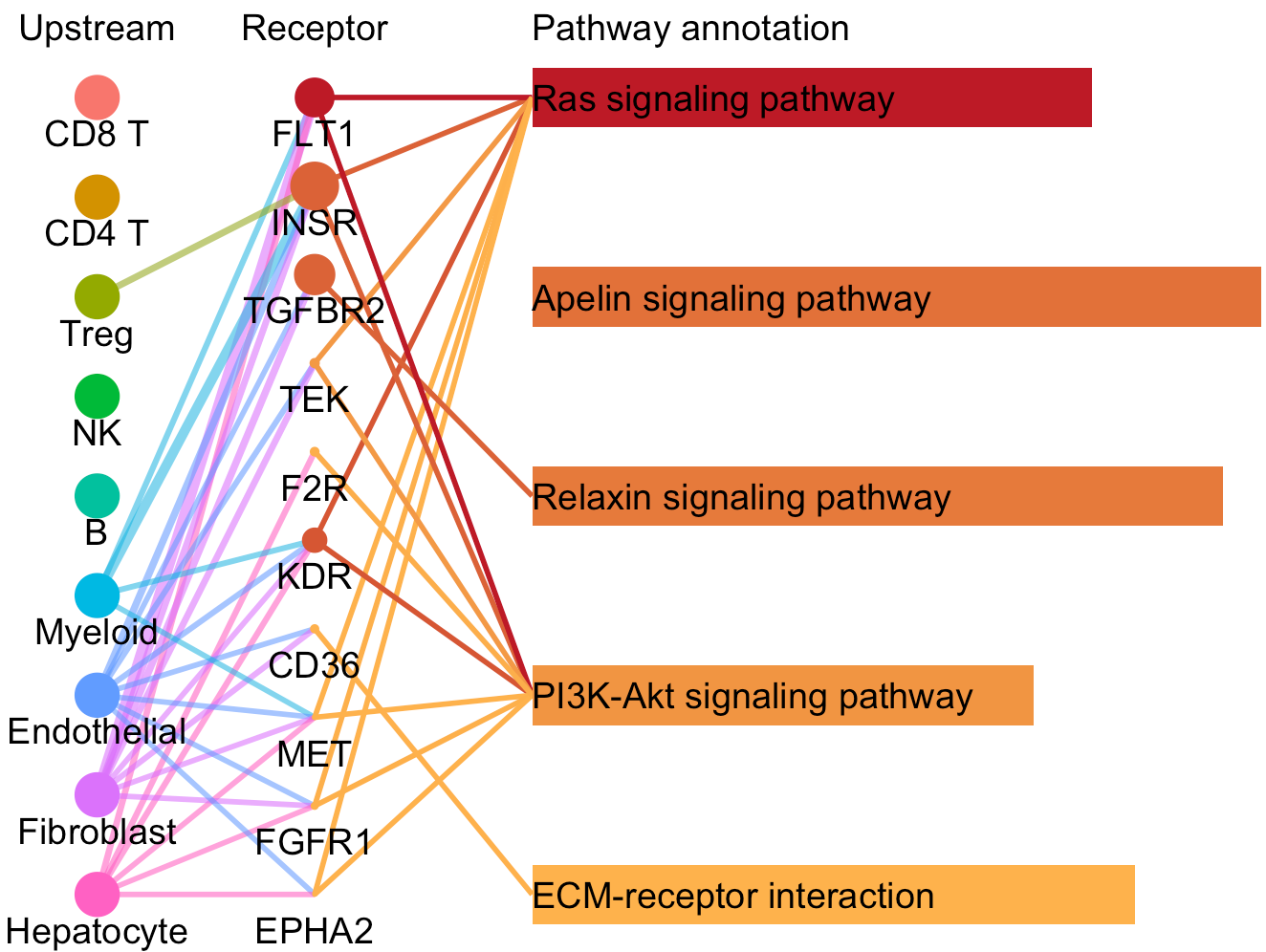
Then network graph tools are to visualize the pathways and associated functional LR interactions.
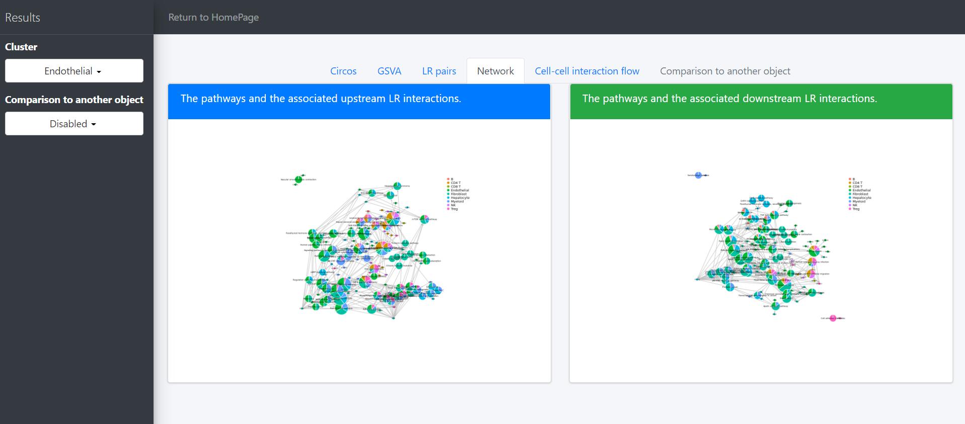
In the above network graph, the pie charts represent the activated pathways in the selected cells (here Endothelial cells) and the scatter points represent the LR pairs of which the receptors are included in the genesets of the linked pathways. Colors of scatter points indicate the upstream clusters releasing the corresponding ligands. Sizes of pie charts indicate their total in-degree and the proportions indicate the in-degree from different upstream clusters.
The legend of the above network graph is generally the same to that of the previous network plot, except that: (i) the scatter points represent the LR pairs of which the ligands are included in the genesets of the linked pathways; (ii) colors of scatter points indicate the downstream clusters expressing the corresponding receptors; (iii) sizes of pie charts indicate their total out-degree and the proportions indicate the out-degree to different downstream clusters.
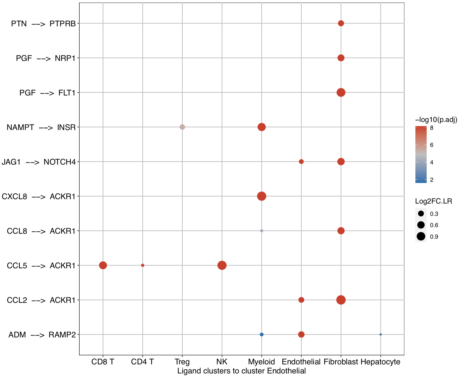
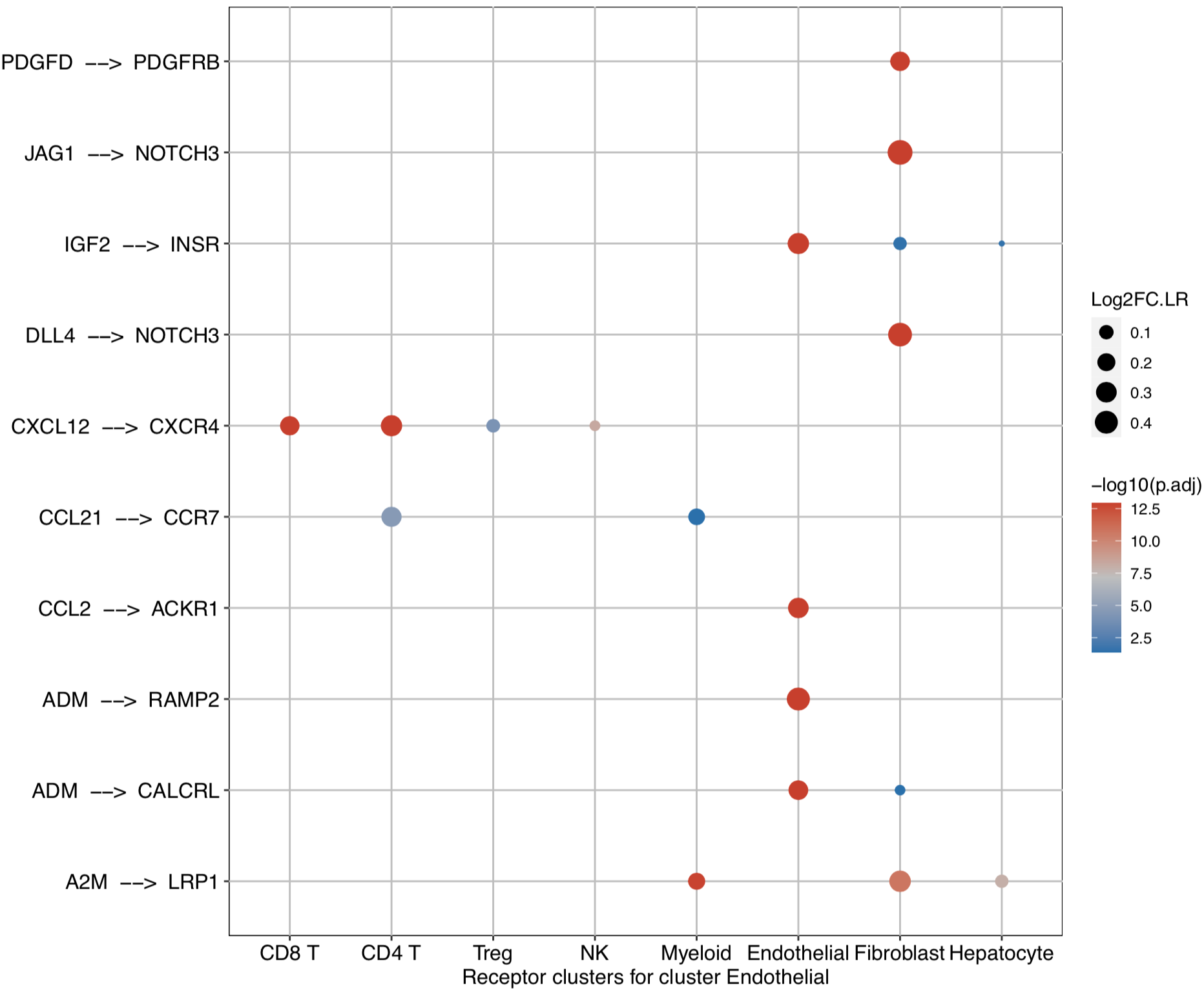
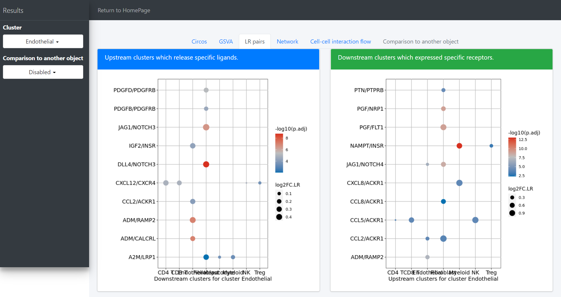
dot plot to investigate the upstream and downstream LR pairs involved in the specific pathways in the selected clusters:
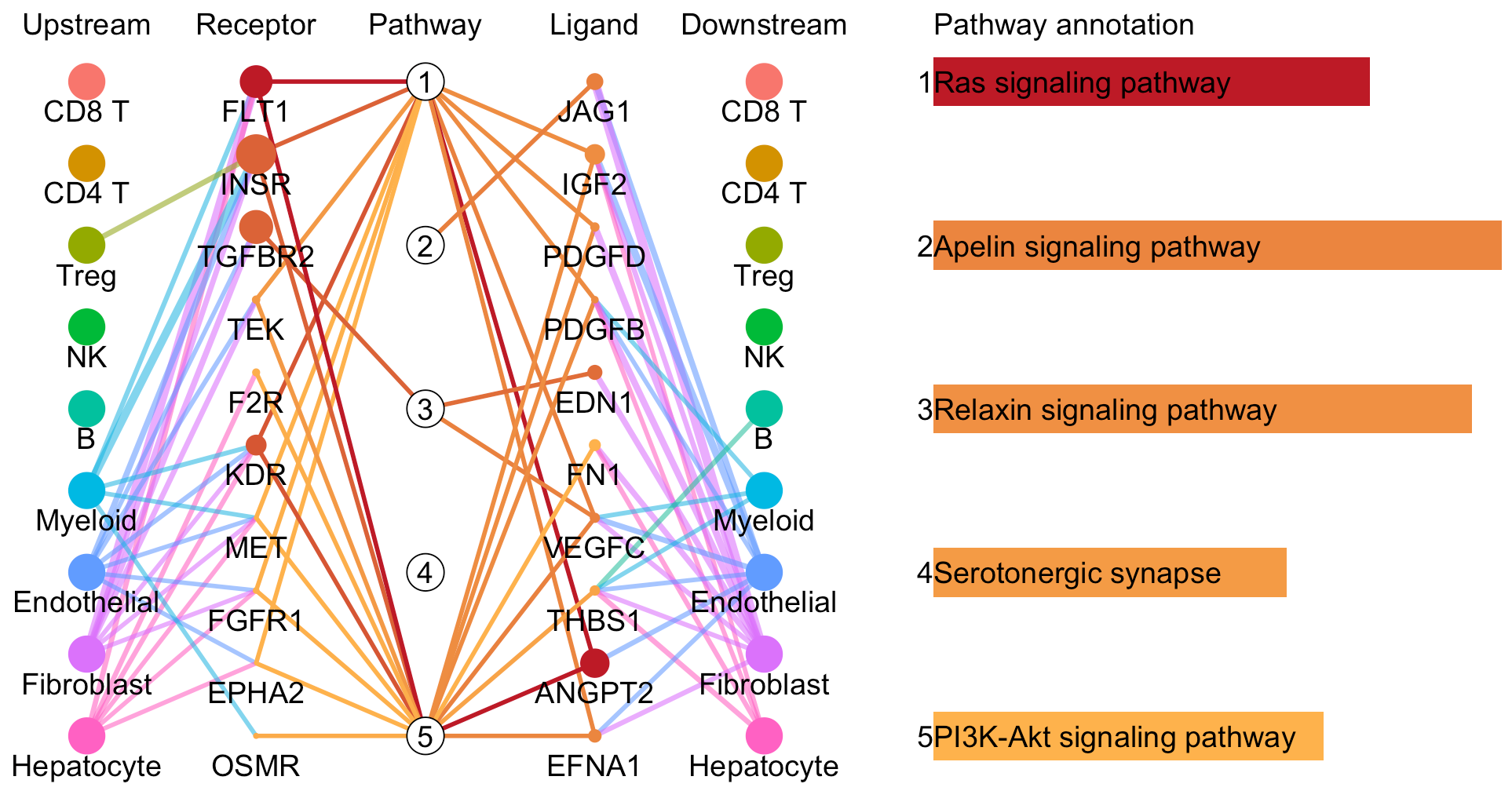
pathway-mediated cell-cell communication chain
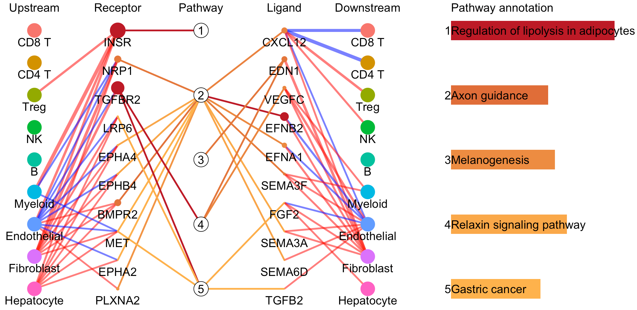
For a specific cell cluster, here named as B for demonstration, CommPath identifies the upstream cluster A sending signals to B, the downstream cluster C receiving signals from B, and the significantly activated pathways in B to mediate the A-B-C communication chain. More exactly, through LR and pathways analysis described above, CommPath is able to identify LR pairs between A and B, LR pairs between B and C, and pathways activated in B. Then CommPath screens for pathways in B which involve both the receptors to interact with A and ligands to interact with C.
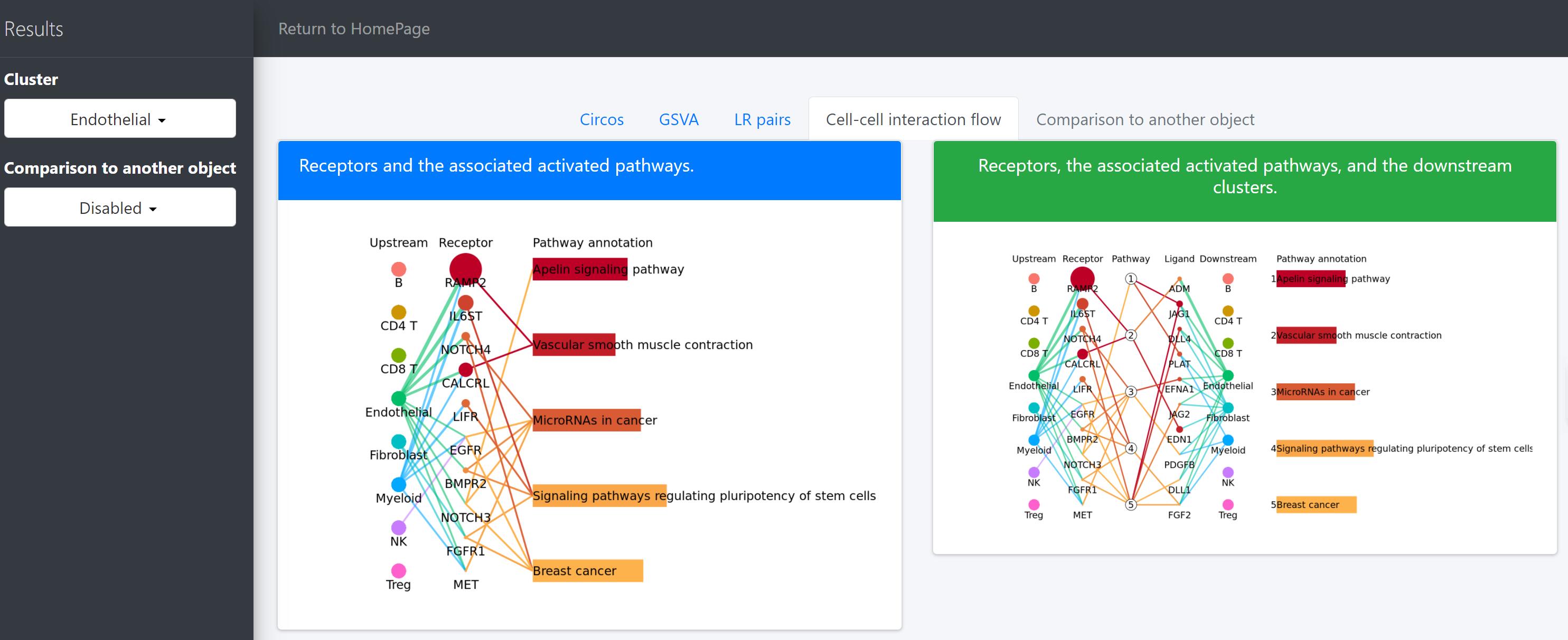
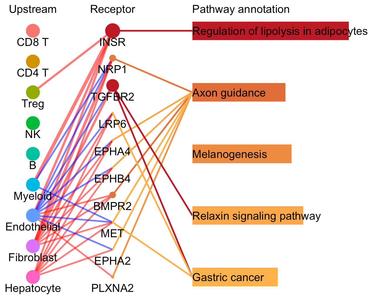
In the above line plot, the widths of lines between Upstream cluster and Receptor represent the overall interaction intensity between the upstream cluster and Endothelial cells via the specific receptors; the sizes and colors of dots in the Receptor column represent the average log2FC and -log10(P) from differential expression tests comparing the receptor expression in Endothelial cells to that in all other cells; the lengths and colors of bars in the Pathway annotation column represent the mean difference and -log10(P) form differential activation tests comparing the pathway scores in Endothelial cells to those in all other cells.
Comparison to another object
“Comparison to another object” tab page, provide useful utilities to compare cell-cell interactions between two conditions, namely case group and control group, such as disease and control. The case group is the current task, and the control group is defined as another task by click “Comparion to another object” drop-down menu. Then, differentially activated signaling pathway-driven cell-cell communications between two CommPath objects is showed.
Here we, for example, use CommPath to compare the cell-cell communication between cells from HCC tumor and normal tissues. We have pre-created the CommPath object for the normal samples following the above steps.
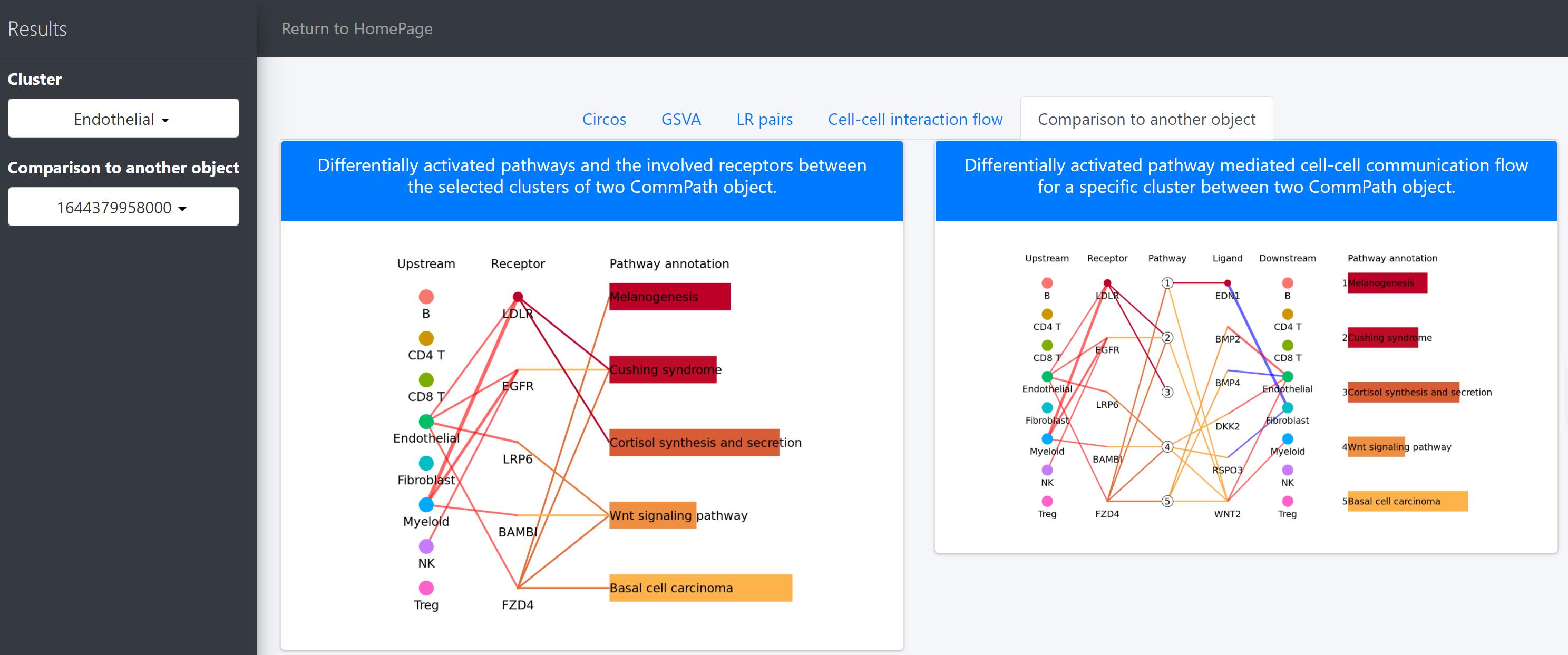
In the above line plot, the widths of lines between Upstream cluster and Receptor represent the overall interaction intensity between the upstream clusters and Endothelial cells via the specific receptors, and the colors indicate the interaction intensity is upregulated (red) or downregulated (blue) in tumor tissues (object.1) compared to that in normal tissues (object.2); the sizes and colors of dots in the Receptor column represent the average log2FC and -log10(P) of expression of receptors in Endothelial cells compared to all other cells in tumor tissues; the lengths and colors of bars in the Pathway annotation column represent the mean difference and -log10(P) of pathway scores of Endothelial cells in tumor tissues compared to that in normal tissues.
4. Download the results
All the results, provided as a zipped package, can be freely downloaded by clicking “Download” buttom on “Task list” section.